Frozenlake 基准测试

在这篇文章中，我们将比较在强化学习 Gymnasium 包中使用 Q-learning 算法的 FrozenLake 环境上，不同地图大小的效果。

依赖项

首先导入一些我们将需要的依赖项。

# Author: Andrea Pierré
# License: MIT License


from pathlib import Path
from typing import NamedTuple

import matplotlib.pyplot as plt
import numpy as np
import pandas as pd
import seaborn as sns
from tqdm import tqdm

import gymnasium as gym
from gymnasium.envs.toy_text.frozen_lake import generate_random_map


sns.set_theme()

# %load_ext lab_black

我们将使用的参数

class Params(NamedTuple):
    total_episodes: int  # Total episodes
    learning_rate: float  # Learning rate
    gamma: float  # Discounting rate
    epsilon: float  # Exploration probability
    map_size: int  # Number of tiles of one side of the squared environment
    seed: int  # Define a seed so that we get reproducible results
    is_slippery: bool  # If true the player will move in intended direction with probability of 1/3 else will move in either perpendicular direction with equal probability of 1/3 in both directions
    n_runs: int  # Number of runs
    action_size: int  # Number of possible actions
    state_size: int  # Number of possible states
    proba_frozen: float  # Probability that a tile is frozen
    savefig_folder: Path  # Root folder where plots are saved


params = Params(
    total_episodes=2000,
    learning_rate=0.8,
    gamma=0.95,
    epsilon=0.1,
    map_size=5,
    seed=123,
    is_slippery=False,
    n_runs=20,
    action_size=None,
    state_size=None,
    proba_frozen=0.9,
    savefig_folder=Path("../../_static/img/tutorials/"),
)
params

# Set the seed
rng = np.random.default_rng(params.seed)

# Create the figure folder if it doesn't exist
params.savefig_folder.mkdir(parents=True, exist_ok=True)

FrozenLake 环境

env = gym.make(
    "FrozenLake-v1",
    is_slippery=params.is_slippery,
    render_mode="rgb_array",
    desc=generate_random_map(
        size=params.map_size, p=params.proba_frozen, seed=params.seed
    ),
)

创建 Q 表格

在本教程中，我们将使用 Q-learning 作为我们的学习算法，并使用 \(\epsilon\)-greedy 来决定每一步选择哪个动作。您可以查看 参考资料部分 以复习一些理论知识。现在，让我们创建我们的 Q 表格，初始化为零，行数为状态数，列数为动作数。

params = params._replace(action_size=env.action_space.n)
params = params._replace(state_size=env.observation_space.n)
print(f"Action size: {params.action_size}")
print(f"State size: {params.state_size}")


class Qlearning:
    def __init__(self, learning_rate, gamma, state_size, action_size):
        self.state_size = state_size
        self.action_size = action_size
        self.learning_rate = learning_rate
        self.gamma = gamma
        self.reset_qtable()

    def update(self, state, action, reward, new_state):
        """Update Q(s,a):= Q(s,a) + lr [R(s,a) + gamma * max Q(s',a') - Q(s,a)]"""
        delta = (
            reward
            + self.gamma * np.max(self.qtable[new_state, :])
            - self.qtable[state, action]
        )
        q_update = self.qtable[state, action] + self.learning_rate * delta
        return q_update

    def reset_qtable(self):
        """Reset the Q-table."""
        self.qtable = np.zeros((self.state_size, self.action_size))


class EpsilonGreedy:
    def __init__(self, epsilon):
        self.epsilon = epsilon

    def choose_action(self, action_space, state, qtable):
        """Choose an action `a` in the current world state (s)."""
        # First we randomize a number
        explor_exploit_tradeoff = rng.uniform(0, 1)

        # Exploration
        if explor_exploit_tradeoff < self.epsilon:
            action = action_space.sample()

        # Exploitation (taking the biggest Q-value for this state)
        else:
            # Break ties randomly
            # Find the indices where the Q-value equals the maximum value
            # Choose a random action from the indices where the Q-value is maximum
            max_ids = np.where(qtable[state, :] == max(qtable[state, :]))[0]
            action = rng.choice(max_ids)
        return action

运行环境

让我们实例化学习器和探索器。

learner = Qlearning(
    learning_rate=params.learning_rate,
    gamma=params.gamma,
    state_size=params.state_size,
    action_size=params.action_size,
)
explorer = EpsilonGreedy(
    epsilon=params.epsilon,
)

这将是我们的主函数，用于运行我们的环境，直到达到最大 episode 数 params.total_episodes。为了考虑随机性，我们还将多次运行我们的环境。

def run_env():
    rewards = np.zeros((params.total_episodes, params.n_runs))
    steps = np.zeros((params.total_episodes, params.n_runs))
    episodes = np.arange(params.total_episodes)
    qtables = np.zeros((params.n_runs, params.state_size, params.action_size))
    all_states = []
    all_actions = []

    for run in range(params.n_runs):  # Run several times to account for stochasticity
        learner.reset_qtable()  # Reset the Q-table between runs

        for episode in tqdm(
            episodes, desc=f"Run {run}/{params.n_runs} - Episodes", leave=False
        ):
            state = env.reset(seed=params.seed)[0]  # Reset the environment
            step = 0
            done = False
            total_rewards = 0

            while not done:
                action = explorer.choose_action(
                    action_space=env.action_space, state=state, qtable=learner.qtable
                )

                # Log all states and actions
                all_states.append(state)
                all_actions.append(action)

                # Take the action (a) and observe the outcome state(s') and reward (r)
                new_state, reward, terminated, truncated, info = env.step(action)

                done = terminated or truncated

                learner.qtable[state, action] = learner.update(
                    state, action, reward, new_state
                )

                total_rewards += reward
                step += 1

                # Our new state is state
                state = new_state

            # Log all rewards and steps
            rewards[episode, run] = total_rewards
            steps[episode, run] = step
        qtables[run, :, :] = learner.qtable

    return rewards, steps, episodes, qtables, all_states, all_actions

可视化

为了方便使用 Seaborn 绘制结果，我们将把模拟的主要结果保存在 Pandas 数据帧中。

def postprocess(episodes, params, rewards, steps, map_size):
    """Convert the results of the simulation in dataframes."""
    res = pd.DataFrame(
        data={
            "Episodes": np.tile(episodes, reps=params.n_runs),
            "Rewards": rewards.flatten(order="F"),
            "Steps": steps.flatten(order="F"),
        }
    )
    res["cum_rewards"] = rewards.cumsum(axis=0).flatten(order="F")
    res["map_size"] = np.repeat(f"{map_size}x{map_size}", res.shape[0])

    st = pd.DataFrame(data={"Episodes": episodes, "Steps": steps.mean(axis=1)})
    st["map_size"] = np.repeat(f"{map_size}x{map_size}", st.shape[0])
    return res, st

我们想要绘制智能体最终学习到的策略。为此，我们将：1. 从每个状态的 Q 表格中提取最佳 Q 值；2. 获取这些 Q 值对应的最佳动作；3. 将每个动作映射到一个箭头，以便我们可以将其可视化。

def qtable_directions_map(qtable, map_size):
    """Get the best learned action & map it to arrows."""
    qtable_val_max = qtable.max(axis=1).reshape(map_size, map_size)
    qtable_best_action = np.argmax(qtable, axis=1).reshape(map_size, map_size)
    directions = {0: "←", 1: "↓", 2: "→", 3: "↑"}
    qtable_directions = np.empty(qtable_best_action.flatten().shape, dtype=str)
    eps = np.finfo(float).eps  # Minimum float number on the machine
    for idx, val in enumerate(qtable_best_action.flatten()):
        if qtable_val_max.flatten()[idx] > eps:
            # Assign an arrow only if a minimal Q-value has been learned as best action
            # otherwise since 0 is a direction, it also gets mapped on the tiles where
            # it didn't actually learn anything
            qtable_directions[idx] = directions[val]
    qtable_directions = qtable_directions.reshape(map_size, map_size)
    return qtable_val_max, qtable_directions

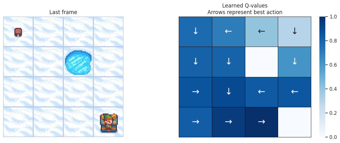
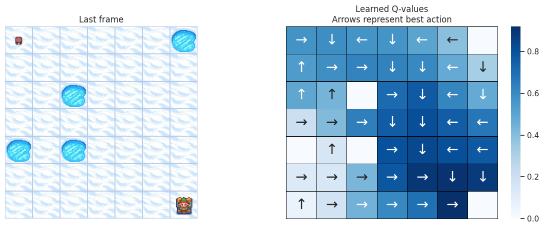
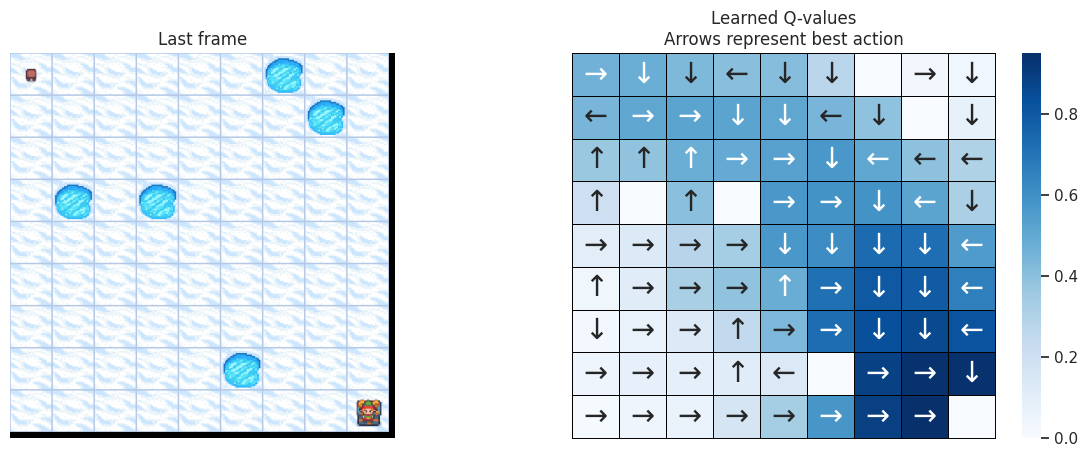
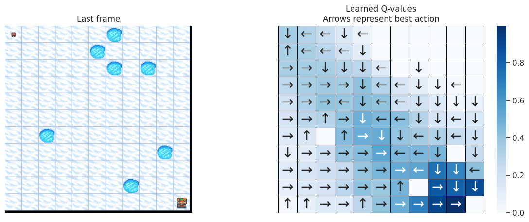
使用以下函数，我们将在左侧绘制模拟的最后一帧。如果智能体学习到了解决任务的良好策略，我们期望在视频最后一帧的宝藏方格上看到它。在右侧，我们将绘制智能体学习到的策略。每个箭头将代表每个方格/状态要选择的最佳动作。

def plot_q_values_map(qtable, env, map_size):
    """Plot the last frame of the simulation and the policy learned."""
    qtable_val_max, qtable_directions = qtable_directions_map(qtable, map_size)

    # Plot the last frame
    fig, ax = plt.subplots(nrows=1, ncols=2, figsize=(15, 5))
    ax[0].imshow(env.render())
    ax[0].axis("off")
    ax[0].set_title("Last frame")

    # Plot the policy
    sns.heatmap(
        qtable_val_max,
        annot=qtable_directions,
        fmt="",
        ax=ax[1],
        cmap=sns.color_palette("Blues", as_cmap=True),
        linewidths=0.7,
        linecolor="black",
        xticklabels=[],
        yticklabels=[],
        annot_kws={"fontsize": "xx-large"},
    ).set(title="Learned Q-values\nArrows represent best action")
    for _, spine in ax[1].spines.items():
        spine.set_visible(True)
        spine.set_linewidth(0.7)
        spine.set_color("black")
    img_title = f"frozenlake_q_values_{map_size}x{map_size}.png"
    fig.savefig(params.savefig_folder / img_title, bbox_inches="tight")
    plt.show()

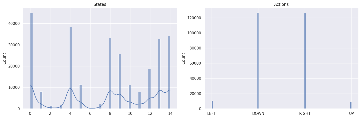
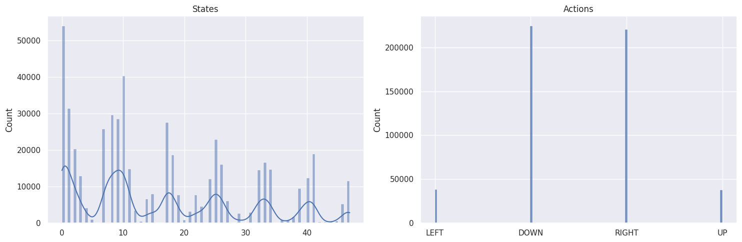
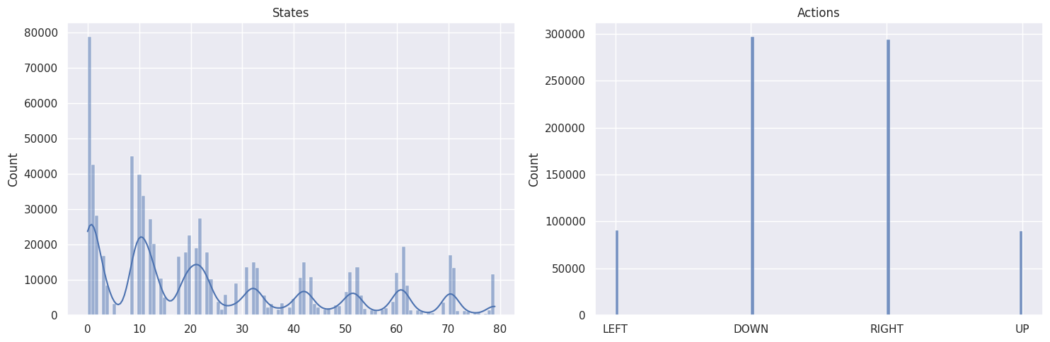
作为健全性检查，我们将使用以下函数绘制状态和动作的分布

def plot_states_actions_distribution(states, actions, map_size):
    """Plot the distributions of states and actions."""
    labels = {"LEFT": 0, "DOWN": 1, "RIGHT": 2, "UP": 3}

    fig, ax = plt.subplots(nrows=1, ncols=2, figsize=(15, 5))
    sns.histplot(data=states, ax=ax[0], kde=True)
    ax[0].set_title("States")
    sns.histplot(data=actions, ax=ax[1])
    ax[1].set_xticks(list(labels.values()), labels=labels.keys())
    ax[1].set_title("Actions")
    fig.tight_layout()
    img_title = f"frozenlake_states_actions_distrib_{map_size}x{map_size}.png"
    fig.savefig(params.savefig_folder / img_title, bbox_inches="tight")
    plt.show()

现在，我们将在几个递增的地图大小上运行我们的智能体：- \(4 \times 4\), - \(7 \times 7\), - \(9 \times 9\), - \(11 \times 11\)。

将所有内容整合在一起

map_sizes = [4, 7, 9, 11]
res_all = pd.DataFrame()
st_all = pd.DataFrame()

for map_size in map_sizes:
    env = gym.make(
        "FrozenLake-v1",
        is_slippery=params.is_slippery,
        render_mode="rgb_array",
        desc=generate_random_map(
            size=map_size, p=params.proba_frozen, seed=params.seed
        ),
    )

    params = params._replace(action_size=env.action_space.n)
    params = params._replace(state_size=env.observation_space.n)
    env.action_space.seed(
        params.seed
    )  # Set the seed to get reproducible results when sampling the action space
    learner = Qlearning(
        learning_rate=params.learning_rate,
        gamma=params.gamma,
        state_size=params.state_size,
        action_size=params.action_size,
    )
    explorer = EpsilonGreedy(
        epsilon=params.epsilon,
    )

    print(f"Map size: {map_size}x{map_size}")
    rewards, steps, episodes, qtables, all_states, all_actions = run_env()

    # Save the results in dataframes
    res, st = postprocess(episodes, params, rewards, steps, map_size)
    res_all = pd.concat([res_all, res])
    st_all = pd.concat([st_all, st])
    qtable = qtables.mean(axis=0)  # Average the Q-table between runs

    plot_states_actions_distribution(
        states=all_states, actions=all_actions, map_size=map_size
    )  # Sanity check
    plot_q_values_map(qtable, env, map_size)

    env.close()

地图大小：\(4 \times 4\)

地图大小：\(7 \times 7\)

地图大小：\(9 \times 9\)

地图大小：\(11 \times 11\)

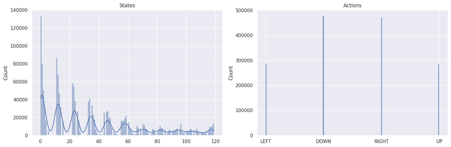
DOWN 和 RIGHT 动作被更频繁地选择，这是有道理的，因为智能体从地图的左上角开始，需要找到通往右下角的路径。而且地图越大，离起始状态越远的状态/方格被访问的次数越少。

为了检查我们的智能体是否正在学习，我们想要绘制累积奖励总和，以及达到 episode 结束所需的步数。如果我们的智能体正在学习，我们期望看到累积奖励总和增加，并且解决任务的步数减少。

def plot_steps_and_rewards(rewards_df, steps_df):
    """Plot the steps and rewards from dataframes."""
    fig, ax = plt.subplots(nrows=1, ncols=2, figsize=(15, 5))
    sns.lineplot(
        data=rewards_df, x="Episodes", y="cum_rewards", hue="map_size", ax=ax[0]
    )
    ax[0].set(ylabel="Cumulated rewards")

    sns.lineplot(data=steps_df, x="Episodes", y="Steps", hue="map_size", ax=ax[1])
    ax[1].set(ylabel="Averaged steps number")

    for axi in ax:
        axi.legend(title="map size")
    fig.tight_layout()
    img_title = "frozenlake_steps_and_rewards.png"
    fig.savefig(params.savefig_folder / img_title, bbox_inches="tight")
    plt.show()


plot_steps_and_rewards(res_all, st_all)

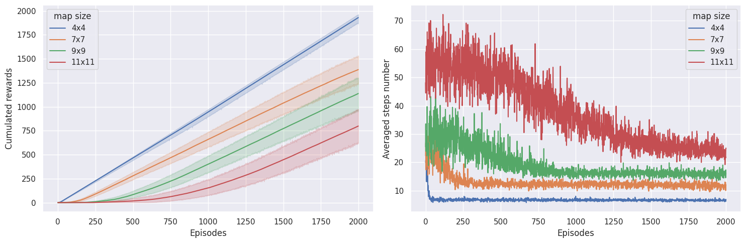
在 \(4 \times 4\) 地图上，学习收敛得非常快，而在 \(7 \times 7\) 地图上，智能体需要 \(\sim 300\) 个 episodes，在 \(9 \times 9\) 地图上需要 \(\sim 800\) 个 episodes，而在 \(11 \times 11\) 地图上，它需要 \(\sim 1800\) 个 episodes 才能收敛。有趣的是，智能体在 \(9 \times 9\) 地图上获得的奖励似乎比在 \(7 \times 7\) 地图上获得的奖励更多，这可能意味着它在 \(7 \times 7\) 地图上没有达到最优策略。

最后，如果智能体没有获得任何奖励，奖励就不会在 Q 值中传播，智能体也就什么也学不到。根据我在这个环境中使用 \(\epsilon\)-greedy 和这些超参数和环境设置的经验，超过 \(11 \times 11\) 个方格的地图开始变得难以解决。也许使用不同的探索算法可以克服这个问题。另一个有很大影响的参数是 proba_frozen，即方格被冻结的概率。如果洞太多，即 \(p<0.9\)，Q-learning 很难不掉入洞中并获得奖励信号。

参考资料

• 代码灵感来自 Thomas Simonini 的 Deep Reinforcement Learning Course (深度强化学习课程) (http://simoninithomas.com/)

• Dissecting Reinforcement Learning-Part.2 (剖析强化学习 - 第二部分)

• David Silver 的课程，特别是第 4 课和第 5 课

• 维基百科上的 Q-learning 文章

• Q-Learning: Off-Policy TD Control (Q-Learning：离策略 TD 控制)，出自 Reinforcement Learning: An Introduction, by Richard S. Sutton and Andrew G. Barto (强化学习导论，作者 Richard S. Sutton 和 Andrew G. Barto)

• Epsilon-Greedy Q-learning (Epsilon-Greedy Q-learning)

• Introduction to Reinforcement Learning (强化学习入门)，作者 Tim Miller (墨尔本大学)